Draw Special Joint
Geometric Nonlinear P-Delta
Move
Click the File menu > New Model command to access the New Model form.
Click the drop-down
list to set the units to ![]() .
.
Click the Grid
Only button  to access
the Quick Grid Lines form. In that form:
to access
the Quick Grid Lines form. In that form:
Select the Cartesian Tab.
In the Number of Grid Lines area
type 3 in the X direction edit box.
type 5 in the Y direction edit box.
type 2 in the Z direction edit box.
In the Grid Spacing area
type 3 in the X Direction edit box.
type 2 in the Y Direction edit box.
type 10 in the Z Direction edit box.
Click the OK button.
Change the units in
the status bar to ![]() .
.
Click the Define menu > Section Properties > Frame Sections command to access the Frame Properties form. In that form:
Click the Add New Property button to display the Add Frame Section Property form. In the Fame Section Property Type drop-down list, select Concrete. Click the Circular button to display the Circle Section form. In that form:
Type ROD in the Section Name edit box.
Click the + (plus) symbol beside the Material drop-down list to access the Define Materials form. In that form:
Highlight the A992Fy50 definition in the Materials list.
Click the Modify/Show Material button to display the Material Property Data form. In that form:
Verify
that the Units
drop-down list is set to ![]()
Verify that the Modulus of Elasticity is 29000.
Verify that Poisson’s Ratio is 0.3
Click the OK buttons on the Material Property Data and Define Materials forms to return to the Circle Section form.
Type 1.5 in the Diameter (t3) edit box.
Click the OK buttons on the Circle Section and Frame Properties forms to exit all forms.
Change the units in
the status bar to ![]() .
.
Click in the window
entitled X-Y Plane @ Z=10 to make sure it is active. The window is
active when the title is highlighted. The screen appears as shown
in Figure E-1.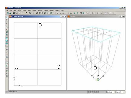
Figure E-1 Screen View Just Before Entering Joints At Elevation Z=10
Click the Draw
Special Joint button ![]() or
the Draw menu > Draw
Special Joint Draw command to access the Properties of Object form.
or
the Draw menu > Draw
Special Joint Draw command to access the Properties of Object form.
Click on the grid intersection
labeled “A” in Figure E-1 to enter a joint at
(0, 2, 10; these coordinates display on the right side of the status
bar).
Click on the grid intersection labeled “B” in Figure E-1 to enter a joint at (3, 8, 10).
Click on the grid intersection labeled “C” in Figure E-1 to enter a joint at (6, 2, 10).
Click the Move
Down in List button ![]() to
move to the X-Y Plane @ Z=0.
to
move to the X-Y Plane @ Z=0.
Click on the grid intersection labeled “D” in Figure E-1 to enter a joint at (3, 4, 0).
Click the Set
Select Mode button ![]() to
exit the draw mode and enter the select mode.
to
exit the draw mode and enter the select mode.
Click the drop-down
list in the status bar to change the units to ![]() .
.
Click in the window entitled 3-D View to activate it. The screen now appears as shown in Figure E-2.
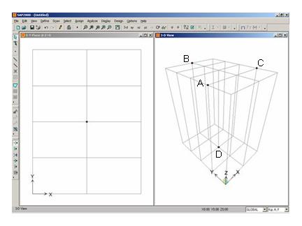
Figure E-2 Screen View After Joints Have Been Entered
Click the Draw
Frame/Cable/Tendon button ![]() or
the Draw menu > Draw Frame/Cable/Tendon
command to access the Properties of Object
form. In that form:
or
the Draw menu > Draw Frame/Cable/Tendon
command to access the Properties of Object
form. In that form:
Verify that the Line Object Type is Straight Frame and that ROD is the selected Section.
In the Moment Releases drop-down list, click on Pinned.
Click on the point labeled “D” and then the point labeled “A” in Figure E-2 and press the Enter key on the keyboard to draw the first rod object.
Click on the point labeled “D” and then the point labeled “B” in Figure E-2 and press the Enter key on the keyboard to draw the next rod object.
Click on the point labeled “D” and then the point labeled “C” in Figure E-2 and press the Enter key on the keyboard to draw the last rod object.
Click the Set
Select Mode button ![]() to exit
Draw Mode and enter Select Mode.
to exit
Draw Mode and enter Select Mode.
Click on the joints identified as A, B and C in Figure E-2 to select them.
Click the Assign menu > Joint > Restraints command to access the Joint Restraints form. In that form:
Verify that the Translation 1, Translation 2 and Translation 3 boxes are checked.
Verify that the Rotation about 1, Rotation about 2 and Rotation about 3 boxes are checked.
Click the OK button.
Click on the joint identified as D in Figure E-2 to select it.
Click the Assign menu > Joint > Restraints command to access the Joint Restraints form. In that form:
Uncheck the boxes for Translation 1, Translation 2 and Translation 3.
Click the OK button.
Click the Define menu > Load Patterns command to access the Define Load Patterns form. In that form:
Type VERT in the Load Pattern Name edit box.
Type 0 in the Self Weight Multiplier edit box.
Click the Add New Load Pattern button
Type LAT in the Load Pattern Name edit box.
Select QUAKE from the Type drop-down list.
Click the Add New Load Pattern button.
Click the OK button.
Select the joint identified as D in Figure E-2 by clicking on it.
Click the Assign menu > Joint Loads > Forces command to access the Joint Forces form. In that form:
Verify VERT is selected in the Load Case Name drop-down list.
Type -750 in the Force Global Z edit box.
Click the OK button.
Select the joint identified as D in Figure E-2 by clicking on it.
Click the Assign menu > Joint Loads > Forces command to access the Joint Forces form. In that form:
Select LAT from the Load Pattern Name drop-down list.
Type 50 in the Force Global X edit box.
Type 0 in the Force Global Z edit box.
Click the OK button.
Click the Show
Undeformed Shape button![]() to
remove the display of joint loads.
to
remove the display of joint loads.
Click in the window entitled 3-D View to activate it.
Click the drop-down
list in the status bar to change the units to ![]() .
.
Click the Select
All button ![]() .
.
Click the Edit menu > Move command to display the Move form. In that form:
Type –3 in the Delta X edit box.
Type –4 in the Delta Y edit box.
Click the OK button.
Click the View menu > Show Grid command to turn off the grid display in the 3-D view.
Click the Run
Analysis button ![]() to access the Set Load Cases to Run form. In that form,
click the Run Now button.
to access the Set Load Cases to Run form. In that form,
click the Run Now button.
When the analysis is complete, check the messages in the SAP Analysis Monitor window and then click the OK button to close the window.
Click the drop-down
list in the status bar to change the units to ![]() .
.
Click in the Deformed Shape window to make sure it is active.
Click the Show
Deformed Shape button ![]() (or
the Display menu > Show Deformed Shape
command) to access the Deformed Shape
form. In that form:
(or
the Display menu > Show Deformed Shape
command) to access the Deformed Shape
form. In that form:
Select LAT from the Case/Combo Name drop-down list.
Click the OK button.
Right click on the bottom joint (the one labeled “D” in the problem statement) to display its displacement. Note the X-direction displacement of this joint. This is the displacement without considering the stiffening effect of the tension in the rods.
Click the Lock/Unlock
Model button![]() to unlock the model.
Click the OK button when asked
if it is OK to delete the analysis results.
to unlock the model.
Click the OK button when asked
if it is OK to delete the analysis results.
Click the Define menu > Load Cases command to access the Define Load Cases form. In that form:
Highlight (select) VERT in the Load Case Name list box.
Click the Modify/Show Load Case button to access the Load Case Data form. In that form:
In the Analysis Type area select the Nonlinear option.
In the Geometric Nonlinearity Parameters area, select the P-Delta option.
Click the OK button to return to the Define Load Cases form.
Highlight (select) LAT in the Load Case Name drop-down list.
Click the Modify/Show Load Case button to access the Load Case Data form. In that form:
In the Stiffness to Use area, select the Stiffness at End of Nonlinear Case option.
Verify that VERT is selected in the Stiffness at End of Nonlinear Case drop-down list.
Click the OK buttons on the Load Case Data and Define Load Cases forms to close all forms.
Click the Run
Analysis button![]() to display the
Set Load Cases to Run form. In
that form, click the Run Now button.
to display the
Set Load Cases to Run form. In
that form, click the Run Now button.
When the analysis is complete, check the messages in the SAP Analysis Monitor window and then click the OK button to close the window.
Click the drop-down
list in the status bar to change the units to ![]() .
.
Click in the Deformed Shape window to make sure it is active.
Click the Show
Deformed Shape button ![]() (or
the Display menu > Show
Deformed Shape command) to access the Deformed
Shape form. In that form:
(or
the Display menu > Show
Deformed Shape command) to access the Deformed
Shape form. In that form:
Select LAT from the Case/Combo Name drop-down list.
Click the OK button.
Right click on the bottom joint (the one labeled “D” in the problem statement) to view its displacement. This is the displacement with the stiffening effect of the tension in the rods considered.